Verifying the Strategy’s Origins

Before diving into my journey, I wanted to confirm the origins of the 3-Bar Triangle Strategy, as I intended to attribute it to Linda Raschke, a renowned trader known for her practical and effective trading systems. After some research, I found that the 3-Bar Triangle pattern aligns with Raschke’s philosophy of identifying high-probability setups using price action and volume, as detailed in her book Street Smarts: High Probability Short-Term Trading Strategies (co-authored with Laurence Connors). While Raschke doesn’t explicitly name this exact pattern as the “3-Bar Triangle” in her writings, the concept of using a short-term consolidation (like a triangle) followed by a breakout with volume confirmation is consistent with her strategies, such as her “Turtle Soup” or “Anti” setups, which often involve breakouts from tight ranges. Raschke frequently emphasizes the importance of volume to confirm breakouts, a key feature of this strategy. Given this alignment, I feel confident attributing the inspiration for this strategy to Raschke, though I’ve adapted it with my own modifications, such as the 20-day MA slope filter.

The Journey: Building the 3-Bar Triangle Strategy

I embarked on this project with a goal: to create my first backtest from scratch, learning the ins and outs of trading strategy development along the way. I chose the 3-Bar Triangle Strategy because it’s a price action-based system that seemed intuitive yet powerful—perfect for a beginner like me to tackle. The core idea is simple: identify a three-bar consolidation pattern (a “triangle”) where the price range narrows and volume decreases, then enter a long trade when the price breaks out above the high of the pattern with strong volume, signaling a potential upward move.

Here’s how the strategy works in its basic form:

• Triangle Pattern: A bar is considered part of a triangle if its high is less than the highest high of the previous two bars, its low is greater than the lowest low of the previous two bars, and its volume is less than or equal to the average volume of the previous two bars.
• Entry: Enter a long trade when the price breaks above the two-day high (the highest high of the last two bars before the triangle) with volume exceeding a rolling average (multiplied by a volume factor).
• Exit: Exit the trade at a take-profit level (a multiple of the stop distance), a stop-loss (the two-day low), or after a maximum number of days in the trade.

I started with a basic Python script using yfinance to download historical data, pandas for data manipulation, and matplotlib for visualization. My initial backtest was rudimentary—it applied the strategy to a single stock (AAPL) over a short period (2020-2023) with fixed parameters. The results were promising but inconsistent, so I knew I needed to optimize and refine the system.

Optimization: Finding the Right Parameters

To make the strategy more robust, I introduced optimization by testing a range of parameters across multiple dimensions. Here are the parameters I optimized, along with their meanings:

• Take-Profit Factor (tp_factor): This determines the profit target as a multiple of the stop distance (the difference between the two-day high and two-day low). I tested values from 1.0 to 3.0 (e.g., 1.5 means the take-profit is 1.5 times the stop distance). A higher value aims for larger gains but risks missing the target if the price reverses.
• Max Days in Trade (max_days_in_trade): The maximum number of days to hold a trade before exiting at the close. I tested 3, 5, 7, 10, and 15 days. Shorter periods reduce exposure but may cut winners short; longer periods allow more time for the trade to work but increase risk.
• Volume Factor (volume_factor): This multiplies the rolling average volume to set a threshold for breakout confirmation. I tested 1.0, 1.25, and 1.5. A higher value (e.g., 1.5) requires stronger volume to confirm the breakout, reducing trades but aiming for higher quality.
• Volume Window (volume_window): The lookback period for calculating the rolling average volume. I tested 3, 5, and 10 days. A shorter window makes the volume filter more sensitive to recent changes, while a longer window smooths out fluctuations.

I used a grid search to test all combinations of these parameters (5 tp_factor x 5 max_days x 3 volume_factor x 3 volume_window = 225 combinations) on the asset GLD (a gold ETF) over the period 2020-2024. To select the best setups, I focused on two metrics: the Sharpe Ratio (for risk-adjusted returns) and Total Return (for overall profitability). I stratified the results by volume_factor to ensure diversity in the top setups, picking the top Sharpe and top Return from each volume_factor group.

Refinements: Adding Filters and Constraints

The initial optimization revealed a few issues: some setups had very few trades (e.g., 3 trades over 3 years), trades were often clustered together, and the results lacked variety in performance. To address these, I made several improvements:

• Minimum Trade Count Filter: I added a filter to exclude setups with fewer than 10 trades, ensuring the strategy was active enough to be meaningful. This increased the trade count to a range of 12-17 trades in my final results.
• Cooldown Period: To prevent trade clustering, I introduced a 5-day cooldown period after each trade, ensuring trades were more evenly spaced across the time period.
• 20-Day MA Slope Filter: To improve the quality of long trades, I added a predictive filter: only take a long trade if the slope of the 20-day moving average (MA) is positive, indicating an uptrend. This filter ensures we’re entering trades when the price is likely to rise, aligning with the strategy’s long-only focus.

Visualization: Plotting the Results

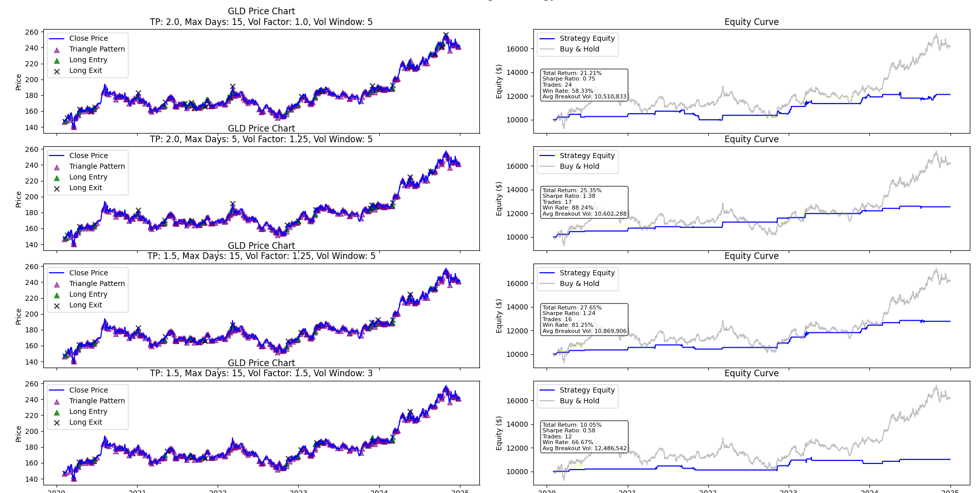
I also worked on visualizing the results to better understand the strategy’s performance. For each top setup, I plotted two charts:

• Price Chart: Shows the asset’s price with triangle patterns (purple triangles), long entries (green triangles), and exits (black X’s).
• Equity Curve: Compares the strategy’s equity curve to a buy-and-hold approach, with key stats (Total Return, Sharpe Ratio, Number of Trades, Win Rate, and Average Breakout Volume) overlaid.

I faced some challenges with the plots—text boxes overlapped, and the charts were initially cluttered. After adjusting the text box position, increasing subplot spacing, the visualizations became much clearer.

Results: Mixed Outcomes with GLD and Beyond

After all the optimizations, I tested the strategy on GLD over 2020-2024. The results were mixed but encouraging:

• Best Setup: One setup (TP: 1.5, Max Days: 15, Vol Factor: 1.25, Vol Window: 5) achieved a Total Return of25% with a Sharpe Ratio of 1.38 % and a Win Rate of 88%. It generated 17 trades, showing a high success rate but modest overall returns.
• Other Setups: Other top setups had Total Returns ranging from 10% to 27%, Sharpe Ratios from 0.58 to 1.24, and Win Rates from 58% to 81%. Trade counts ranged from 12 to 16.

I also tested the strategy on other assets, including stocks (like AAPL) and indices (like QQQ). The results were similarly mixed: the strategy was profitable in most cases, with Win Rates often above 60%, but it didn’t consistently outperform a simple buy-and-hold approach. The strategy’s strength seems to be its consistency (high Win Rates) rather than outsized returns.

Reflections: Struggling with Interpretation

While I’m proud of building this backtest from scratch, I’ve struggled a bit with interpreting the results. The high Win Rate (up to 88% for GLD) is exciting, but the Total Returns are modest, especially compared to buy-and-hold for more volatile assets like QQQ. I’m not sure if the strategy’s conservative nature (fewer trades, focus on uptrends) is a strength or a limitation. The Sharpe Ratiosare decent but not exceptional, and I’m unsure how to balance the trade-off between risk-adjusted returns and overall profitability. I also wonder if the strategy is better suited for certain market conditions (e.g., trending markets) or assets (e.g., less volatile ones like GLD).

Next Steps

This journey has been a huge learning experience, and I’m excited to share it with others. I plan to continue refining the strategy—perhaps by testing additional filters (like ADX for trend strength) or exploring other systems from traders like Linda Raschke or Larry Williams. I’d also love to hear feedback from the community on how to interpret these results and improve the strategy further.